In our
previous post, we explored different ways to interpret a
relation. We showed how a relation could be viewed as a table, as a set of facts, as a predicate function, as the generalization of a function, and as subset of a cartesian product.
These interpretations provide us the ability to rise above marketing and technologies and see the underlying abstraction for what it is. There are important lessons that can be derived from following this path, of separating abstraction from implementation:
that relations/tables are everywhere and not just within a database
that in fact a database can be understood on a sliding scale from in situ to curated ( “schema on read” versus “schema on write”), and just like relations a database can be ‘everywhere’ (this will be the subject of a future post)
that relations are fundamental, abstract, and omnipresent (like types)
that relations have many different pedagogical manifestations, (as we listed above and covered in the previous post)
that relations provide an interesting way for understanding many very different technologies, from logic programming languages, to semantic databases, to graph databases, to various different NoSQL-ish things, to SQL, Hive, and Pig.
These themes (more opinions) evolved during my years of exposure to the Big Data world as a way to contextualize the exploding menagerie of technologies. I have been grateful to the Big Data world for showing me that the world of databases is neither a dry, nor solved, problem and that databases, knowledge-bases, logic, etc., are all interrelated in ways deeper than previously expected (or at least deeper than I previously expected).

Let’s Get Practical

There is an unfortunate tendency in the IT community to belittle something by calling it non-practical when it tends to be 1) not popular and 2) theoretical. To counter this charge, and to appeal to as large an audience as possible, let’s immediately dive into answering a very practical problem. As we go through this example, we will adopt the interpretation that a relation is a table. This is a very practical manifestation of our hidden relation, but will also be a long discussion.
The Problem Statement: Let us count the number of different browser types that have visited a website by scanning an Nginx log file.
As we tackle this problem, we will show this answer as a series of relational operators manipulating relations using Unix command lines.
In the above snippet of configuration, somebody has set up their NGINX (or maybe Apache) webserver to log to disk each HTTP interaction with the website. The log file looks like this:
127.0.0.1 - - [19/Jun/2012:09:16:22 +0100] "GET /GO.jpg HTTP/1.1" 499 0 "http://domain.com/htm_data/7/1206/758536.html" "Mozilla/4.0 (compatible; MSIE 7.0; Windows NT 5.1; Trident/4.0; .NET CLR 1.1.4322; .NET CLR 2.0.50727; .NET CLR 3.0.4506.2152; .NET CLR 3.5.30729; SE 2.X MetaSr 1.0)"
The practicality just oozes from the page.
The answer that got accepted was one of those Jedi like answers that showed the power of true Unix mastery:
cat /var/log/nginx-access.log | grep "GET" |
awk -F'"' '{print $6}' | cut -d' ' -f1 |
grep -E '^[[:alnum:]]' | sort | uniq -c | sort -rn
It is interesting to look at these individual commands as part and parcel of the Unix philosophy. But it’s also interesting to look at these as manifestations of relational operators, as originally described by Codd.
The Unix Pipe World According to Relational Algebra
Diving straight in, we can enumerate what is happening as a chained composition of the following relational operations:
first we create an un-named, one column relation by invoking cat,
next we horizontally subset (select operator) some of the tuples and produce a new relation
next we vertically subset (project operator) the sixth column, producing a new relation again
next we vertically subset (project operator) the first column. New relation again
we select again. New relation again
then we sort (strictly speaking this shouldn’t matter in the idealized tuple world that Codd first described)
next we do a group-by and a count, new relation again
finally we sort again, final relation
For those interested, let’s go through each one of these steps in more detail.
First: Create a boring nameless Relation...
cat is the Unix command line to output the contents of a file to standard out. By doing this, we have implicitly created our first relation, a table with a single column. In reality, neither the relation nor the column have explicit names, (but nothing prevents us from giving them automatic names based on their position from the ‘left’ or the ‘right’ -- naming, while an important step, can be automated).
 This first relation consists of tuples that represent each line in the file, and the type of this singular column is a string (or varchar or chararray, etc). Not to belabor a point, but this is absolutely a relation, no matter how primitive, un-named and un-indexed it might seem. Do not confuse abstractions with implementations (this might, in fact, be the overarching theme for this entire series of posts). The relation exists in our minds as a means of understanding something physical and tangible. The relation is a product of our interpretation. In the Big Data world, we call this late-binding of interpretation “Schema on Read” indicating that our schema (another word for interpretation) is decided when we read it from disk, and not when we write it to a system.
Second: Generate a new Relation using the Selection Operator (i.e. grep for matching lines)
grep is the unix command line that takes a line oriented data and removes (or keeps) those lines that match the given regular-expression predicate. In this example, our regular expression matches the exact string “GET” and keeps those tuples that match, thus providing a horizontal subsetting operator.
Let’s repeat what we have done here: we have transformed one relation (the original contents of the file as produced by cat) into another relation by using an operator. This is why Codd called one half of his study of the relational model ‘an algebra’ in his 1972 paper (Codd, E.F. (1970). "Relational Completeness of Data Base Sublanguages". Database Systems: 65–98.).

Specifically, we have used what is now called the unary selection operator to create one relation from another. For those of you following along with a crush on SQL, this is exactly the same as doing something like :
select * from FILE
where contents = “%GET%”
(the WHERE clause is highlighted in green and shows the syntactic manifestation of the selection operator σ in the SQL language)
Third: Project out only the Data we are Interested in
Even people familiar with Unix will bow down before the impressive power of ‘awk’. In the following snippet of awk, we are using the command line switch ‘-F’ to indicate what is our delimiter between fields. Specifically, we have asked awk to use the double-quotes character, and to make as many fields as there are delimiters +1. It turns out, in the case of this NGINX log file, that there will be six fields separated by five double-quote characters. Our awk command then prints out the sixth column. You can see that the result should be a vertical subset of our original line.
At this point, you can see that we have really done two things:
we have re-interpreted the original relation by applying a new schema and in doing so have generated a new table/relation of six columns
we have asked awk to only pass through the sixth column, and thus have generate a new table/relation
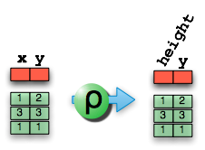
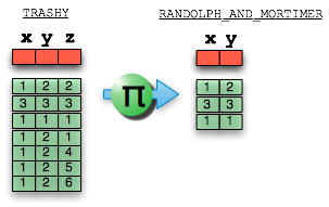
This second point is the application of the projection operator, fondly known as pi (π). The vertical sub-setting of a relation, to create a new relation, will change the schema and remove dimensions. This is shown in the following graphic where a table of two columns: x and y, has the ‘y’ dimension projected out.
For those of you following along with a crush on SQL, this is exactly the same as doing something like:
select user_agent from GET_RECORDS
(the highlighted green shows the syntactic manifestation of the projection operator π in the SQL language)
Let’s Take a Break

We said we would veer into the realm of practicality. However, even this discussion was rife with all sorts of mathematical concepts of dimensions, and algebras, and operators… Let’s sum up the practical points then
relations provide us a way to think about our data
grep is like the “where” clause in a SQL statement… it subsets horizontally, and keeps the schema the same
awk (with a print $6 command) can be like a projection operator, or like selecting a column from a table, and it changes the dimensionality of our data
UNIX pipes are awesome
On the Road Again

So far, in this example, we have been treating a relation as if it were a table with rows/tuples and columns/dimensions. We might as well finish up the last few steps, but for those of you who want to get onto the next example, you can always skip past these last sections and see how relations can be found in shadows, when relations are a subset of a cartesian product. To review these concepts, please see the previous post: “What the Heck are Relations?”
Four: Get the Browser Type from the User Agent using Spaces
cut is another unix command that does what awk does. It has different syntax and the choice of awk over cut may be one of convenience and/or familiarity. At this point, we have used the -d switch to say that the space character has become our new delimiter. In the above graphic, we can see how the User Agent text (a payload from the HTTP header) has been split, and we have isolated our first column, which is the actual browser and version (see Section 14.43 of RFC 2616 (HTTP/1.1)).
In the above graphic, the result of this command for this row will be the text “Mozilla/4.0”. We are getting close to what we need.
Five: Remove those Garbage Rows/Tuples that are clearly not real Browsers
This is a maintenance step to get rid of all those garbage lines that come from bad user agents. When you are exposed to the wild wild world of the open internet, there’s nothing stopping somebody from sending weird values for the User Agent. At this point, we implement a heuristic that says that only browser versions beginning with alphanumeric characters are allowed.
Six: Sort so that the following uniq operator will work 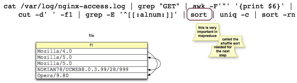
Sort is an interesting “operator”. I have purposely put the term operator in quotes because the original mathematics behind Codd’s Relational Model made no claim about ordering. In fact, ordering a relation does not change the equality semantics of that relation (according to the model) as ordering is irrelevant in set-based models. One may even posit that the only need for ordering is to provide an easy to read listing for human consumption.
Tangent: The other interesting thing to note here is that we have to do this because we know a priori that the following UNIX command uniq will only group and coalesce contiguous rows. So we are doing a necessary step based on the “limitations” of uniq. And while this practical bit of hackery breaks our beautiful model, it does have a nice implementation analog to the MapReduce machinery of Hadoop which needs to provide a shuffle/sort before giving data to a reducer.
|
Seven: Run the uniq command to do a GroupBy and Count
Hit the man page for uniq and you will see that using the -c switch does a group-by and a count. For those of you who love SQL, this is like
select count(browser_type) from browser_records
group by browser_type ;
Tangent: To be honest, I am not sure how Codd’s original work treated GroupBys as operators. However, in Pig, which permits Zeroth normal form data, this is essentially two operations: an initial GroupBy operator that turns the original relation into a hard-coded two-column relation with the group key and a bag of the partitioned rows nested within the cell. Then a count UDF on a FOREACH operator, which is essentially an extended projection semantic.
|
Eight: A final sort for the benefit of us Humans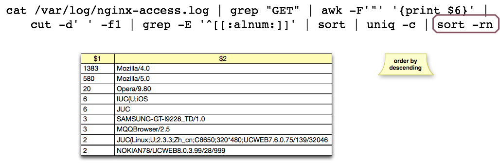 Finally, and to wrap this up, we provide a final sort operator which allows us to see the browsers with the most hits at the top.
And the analogous SQL:
select bcount, browser_type from browser_counts
order by bcount desc ;
Tangent: Horizontally Scaled Implementation -- a Practical Pig Program 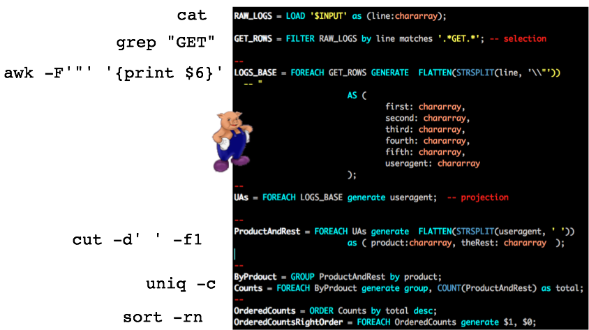
In the above graphic, I am showing an alternate and real implementation of our UNIX operators using Apache Pig (a relational language built atop Hadoop). This is an actual Pig program that does the same thing as these UNIX commands. The difference, of course is obvious: while the UNIX command lines are run on a single CPU and might run for days if this NGINX file is terabytes large, the Pig program compiles down to MapReduce tasks which spawn mappers and reducers on cluster nodes to implement the abstract relational operators and may effectively parallelize this embarrassingly parallel problem -- i.e. horizontal scalability.
The nearly one-to-one mapping between the Unix command line and the Pig code is not accidental. I purposely chose the UNIX example as a way to explain how Pig works. Most people who have never seen Pig but only worked with SQL find that the syntax is difficult to swallow. The entire UNIX command line example was addressed to gently introduce the idea of a step-wise transformation operator syntax. Again, I don’t think Pig gets enough love.
|
Finishing Up: How far we have come. Where we can go.
At this point, we have provided a relational explanation for this hard example of parsing an NGINX log file. It was a practical example, and showed us that there is some applicability to the abstract terms we have developed thus far.
For a more theoretic view of what’s going on, please see the previous post where considered the many different manifestations (or interpretations) of the word relation. This will be a fun discussion and will give us an inkling into how so many different systems could provide their own twist around storing data. If we do our job correct, then we will have a holistic view where we understand data as knowledge, rows/tuples as facts, and NoSQL technologies as access-oriented implementations that have chosen a particular access-vector over another. RDF triples, graph databases, datalog, document databases, key-value databases: no matter how inverted or how materialized for other access-patterns, the underlying relation is present.
Another Concrete Example: Steganographical Shadows
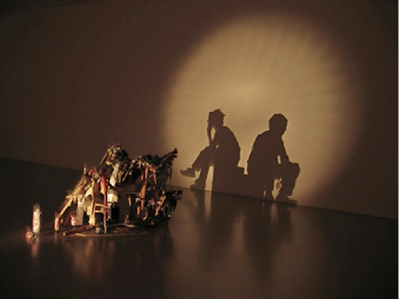
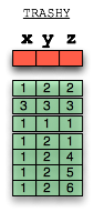
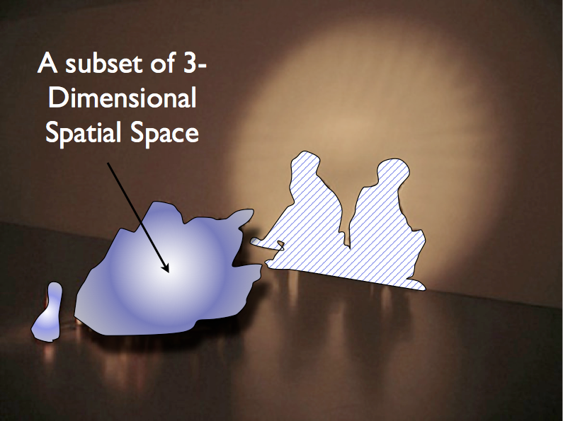
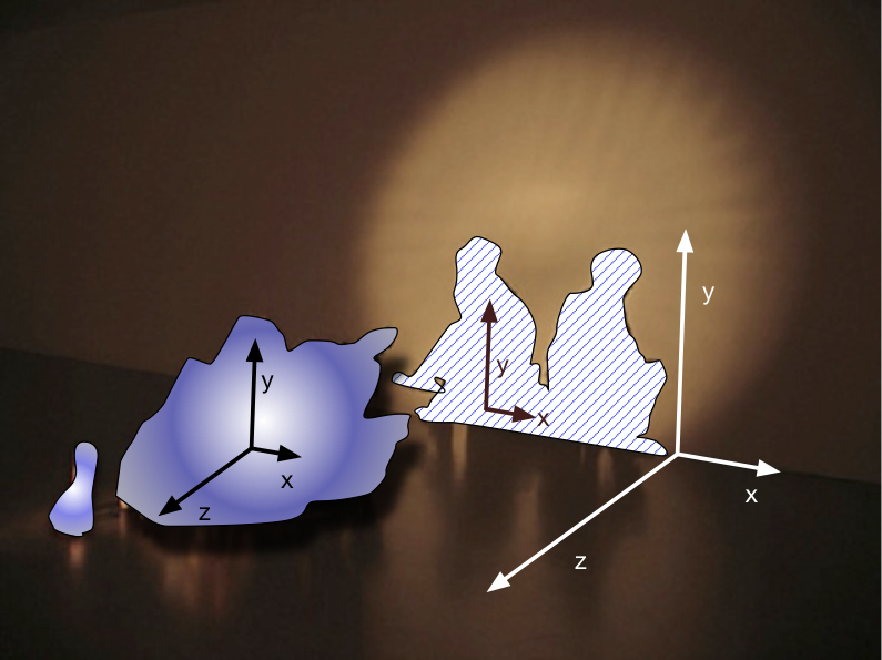
Given the historical journey of abstraction we just surveyed, it would be great fun to show one more last concrete example of a relation. One might say that the overriding theme of this and previous posts is not to confuse abstraction with implementation. To drive home this last point, we take the notion of a relation as a subset of a cartesian product to a very very concrete place, the real world that you and I live in, the world of three actual (debatable) spatial dimensions, in which x, y, and z mean width, height, and depth. The world in which my body occupies a subset of cartesian points, and has extent and boundaries. A world in which every object is a subset of the entire universe.

 If we ever do try to adopt extra glyphs for a > base-36 system. I suggest the one above (hereafter known as the Eklund Encoding), as it makes lambda the answer to life, the universe, and everything.